By Patrick Schwager

Now the new season starts and the question is how to optimize fieldwork. During the past week I have been thinking about the sampling design for a number of new species that will be included in species distribution models (SDM). The aim is to find new occurrence sites of this species within the Styrian Alps. A variety of meaningful site properties need to be incorporated in SDMs to cover the whole range of the species’ preferences. The process for the random selection of sampling sites shall also be automated within an R script in order to avoid making the redundant steps by hand.

A lot of strategies for sampling design can be found in the scientific literature, e.g. random sampling or the gradsect approach. The latter uses an environmental gradient within the study area and randomly choose sites within a transect (25 km width) that crosses this gradient.

The mapping project of vascular plants in Austria provides occurrence information with a resolution of 6.25 x 5.55 km (grid cells). This dataset could be used to portray the environmental gradient of the known species range. Additional information about height and aspect is also needed to detect variations of occurrence based on terrain. This can be derived from a digital elevation model (DEM).

The following steps are necessary to identify different sampling sites of species of interest (Primula glutinosa), including altitude-aspect classes and known range of occurrence:

Step 1: Select only grid cells with known occurrence of Primula glutinosa.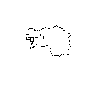
Step 2: Generate altitude classes of 200 m steps and aspect classes (table 1) derived from the DEM. Then combine this information by intersection and select only areas above 1600 m that are greater than 1 hectare.

 

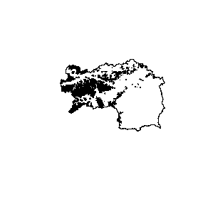Table 1: Classification of aspect.

Direction	Class	Degrees [°]
Flat	1	no direction
North	2	0-22.5
Northeast	3	22.6-67.5
East	4	67.6-112.5
Southeast	5	112.6-157.5
South	6	157.6-202.5
Southwest	7	202.6-247.5
West	8	247.6-292.5
Northwest	9	292.6-337.5
North	10	337.6-360

 

Step 3: Because I am interested only in areas where Primula glutinosa is known, I reduce the polygons from step 2 using the grid cells of Primula glutinosa of step 1.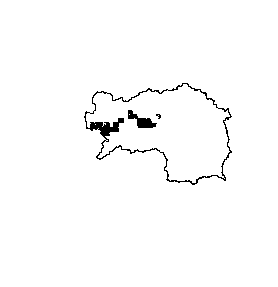
Step 4: From the resulting polygons I randomly select 200 and calculate the center points. Then I export these points as *.gpx files to load them in GPS devices or use them to make field maps for the survey.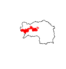

Of course, 200 points is very ambitious, and many of them will not be visited or lie in habitats that are not suitable for the species (e.g. forests). However, with a higher number of sampling points I can easily choose another point if one point cannot be reached and thus reduce field trips without sampling success.

Finally, I want to check whether the altitude and aspect classes are equally represented (step 5 and 6). This is important for the SDMs taking all possible altitude-aspect variations into account. Some altitudes are not optimally represented in the samplings points. Aspect shows better results. Though, north faced areas (class 2 and class 10) are a little bit under represented. I have to keep this in mind in the field and if possible make some additional sampling for missing classes.

Step 5: Altitude classes within the sampling sites.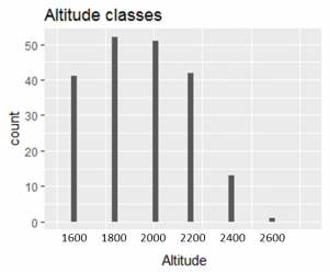
Step 6: Aspect classes (exposition) within the sampling sites.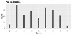
Step 7: Subset of sample points in the “Schladminger Tauern” at Klafferkessel.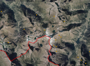